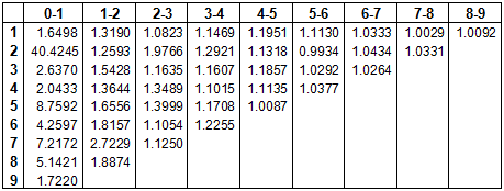
Mack (chain ladder) is volume-weighted average link ratios

When we compute a ratio, y/x, what are we looking at?

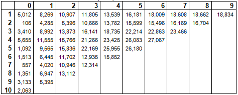
Data are incurred losses from Mack (1994).

Consider the ratio of the cumulative value in AY1, DY1 to the previous value in AY1:

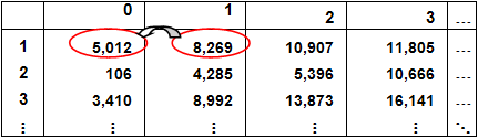
8269/5012 = 1.65

Let's call the number on the numerator y and the number on the denominator x.

Let's look at a graph of DY1 vs DY0. What is the value 1.65?

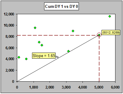
If you plot x and y as a point on a plot, the ratio y/x is the slope of the line through the origin that passes through that point.

When we think of there being a "typical" ratio (which we may want to use for prediction), we are also talking about a "typical" slope through the origin on that (x,y) plot.

If our measure of "typical" is some kind of average (such as a weighted average, a geometric mean, an average of the most recent values, or whatever), we are talking about both an "average" ratio and at the same time, an "average" slope.

In statistical terms, we're using sample ratios to estimate the underlying ratio, since the observed ratios are "noisy".

We are also saying that, given the previous cumulative, we expect that on average the next cumulative is a multiple of the previous one. That is: E(y/x | x) = r is equivalent to E(y | x) = rx.

"E()" stands for "expected" (underlying average) value of whatever is in parentheses, and "|" means "given". So E(y|x) means "the expected value of y, given the value of x".

The left side is a ratio, r, the right side is a line through the origin with slope r. They both describe the same relationship between one cumulative or incurred and the next.

So if there's an underlying "ratio", it's also an underlying slope.

Here's one such "average" line, an ordinary regression line through the origin:

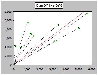
The slope of this line is around 2.217, which is an estimate of the underlying ratio.

Residuals

The residuals from this fit are the differences between the points and the line. Residual = data - fit of method ; Residual trend = data trend - method trend We use residuals to assess ways in which the model assumptions don't apply.

Let's calculate the residual for the point with y = 8992 and x = 3410, and for the point with y = 9565, x = 1092 (these are from AYs 3 and 5 respectively). The observed value for DY1 for the point circled in red below is 8992.

The fitted value (the height of the line at the x-value 3410) is 3410 x 2.217 = 7560.

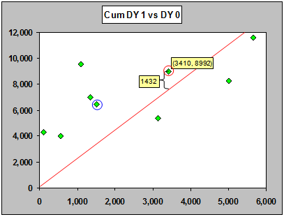
The residual, 1432 is 8992 - 3410 x 2.217; the observed value in DY 1 minus the prediction from the ratio times the previous value (residual = data - fit). The observation with the largest residual is circled in blue. Its observed (y) value is 9565, while the x value is 1092. Consequently, its residual is 9565 - 1092 x 2.217, which gives 7144.

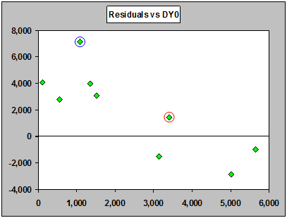
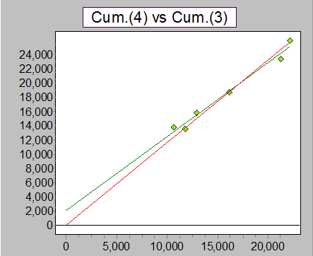
Above are residuals from the fitted line (ratio). Notice the downward trend! Something is clearly amiss; the line through the origin doesn't describe the relationship well. In fact, the residuals are getting smaller as the previous cumulative gets larger. Look at the fitted line again, and see how the points on the left are above it and the points on the right are mostly below it. The relationship is not a line through the origin:

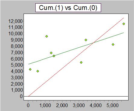
Above is a line of best fit in green. Clearly a line that doesn't go through the origin is a better description of the relationship here.

Normally residuals are divided by their (individual) standard deviation, so that they share a common scale - the result is standardized residuals. Secondly, it's important to see whether the residuals are related to other likely predictors of the observations (in which case we will see non-random trends in the residuals plotted against those predictors). One obvious thing to do is to look at residuals against the three directions (accident year, development year and calendar year), as below. The fourth plot, residuals vs fitted values, is a standard regression diagnostic. Notice that it has exactly the same appearance as the above plot - only the scale labels are different!

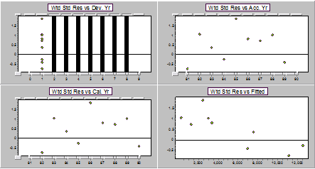
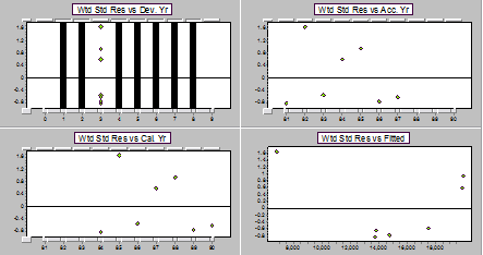
Residual display for a ratio model for DY1 on DY0 (first pair of years).

The plot against accident and calendar years are the same because we only have a single pair of years. There's also not a lot of information in the residuals for a single pair of years - patterns have to be quite strong for us to be able to pick anything up.

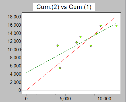
Here's the plot of y vs x for the second pair of years (DY2 vs DY1), followed by the corresponding residuals.

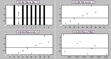
Residual display for a ratio model for DY2 on DY1 (second pair of years).

In the model for DY2, we can see an increasing trend against calendar (and accident) year, and a decreasing trend against fitted values - again, the relationship between DY2 (y) and DY1 (x this time) is not through the origin.

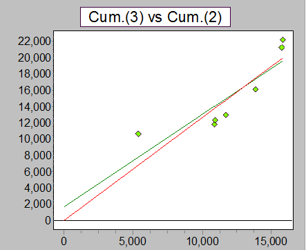
Plot of y vs x for second pair of years (DY3 vs DY2).

Residual display for a ratio model for DY3 on DY2 (third pair of years).

Plot of y vs x for third pair of years.

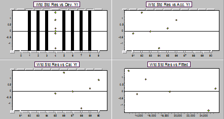
Residual display for a ratio model for DY4 on DY3 (fourth pair of years).

By now it's getting hard to see much of anything going on, there are only 7 and 6 points respectively in the most recent two sets of residual plots above.

We can combine the residuals together into a display against each direction. The plots against accident and calendar years will no longer be redundant, and we will be able to pick up trends in those directions. Note that the plot against development years will not show lack of fit in general, since the fitted line will go through a "weighted average" value of y at each development, but it will allow us to see what's going on with the spread around the line. An overall trend in the residuals plotted against fitted values shows that it is highly likely an intercept is needed.

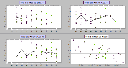
We can see a strong overall downward trend against fitted values. This strongly suggests a need for an intercept term!

The standard chain ladder ratio (Mack)

The standard chain ladder ratio (Mack ratio) is a kind of weighted average of the ratios, where the weight is the previous cumulative - it's sometimes called a "volume weighted average".

An ordinary average of a set of y values (y1, y2, ... yn) is (y1 + y2 + ... + yn)/n. We can write that in short form as:

A weighted average has a weight for each observation, so that an observation with more weight "affects" the average more than one with less weight. It "pulls" the average toward it. A weighted average looks like this:

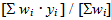
A weighted average ratio is written like this:

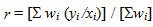
The chain ladder/Mack model has wi = xi .

That is,

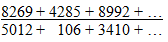
In other words, if we add up the two columns and take the ratio to get the chain ladder ratio,

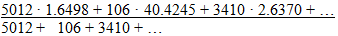
it's the same as weighting the individual ratios by the first column and taking the average:

There are three entirely equivalent ways of looking at the same thing - as a ratio of sums, and a weighted average ratio, and as a weighted average slope (weighted regression line through the origin).

Because the weights applied to the ratios are the previous value (incurred or cumulative), this kind of weighted average is often called a volume-weighted average ratio.

Mack (chain ladder) is volume-weighted average ratios

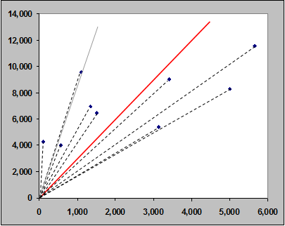
Individual ratios and the standard chain ladder (Mack) ratio (red) for DY1 vs DY0. The arithmetic average of the ratios is in gray.

Below are the residuals for the Mack model applied to all pairs of years.

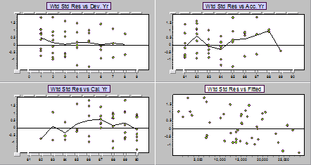
Again, we see a strong downward trend. Note that if a line through the origin is inadequate because the actual relationship needs an intercept, then no other line through the origin will fit. That is, no ratio, no matter how you choose it, will adequately describe the development.

Section II. Mack method (volume-weighted average link ratios) does not distinguish between accident and development years is available here