There are several related reasons why the link ratio methods commonly used for forecasting outstanding claims don’t work. This note addresses a couple of those reasons. Link ratio methods obscure very important trend changes. Link ratios cannot capture the trends in the data. Indeed, link ratios can’t even tell the difference between two arrays when the only difference is a simple trend change. If you cannot identify important trend changes in the past, and don’t know the trend that your forecasting method has already built in for the future, you cannot make informed assessments about the suitability of your forecasts nor can you see how to correctly adjust them in the light of other information.
These simple ideas are first illustrated with a simple series of oil prices.
Trends in a single series of numbers
Let’s look at a familiar series, oil prices. The figures come from the Energy Information Administration website and represent the Refiner Acquisition Cost of Imported Crude Oil between 1994 and 1996.
To visit the Energy Information Administration web site click here.
The actual numbers are in a table at the end of this page.
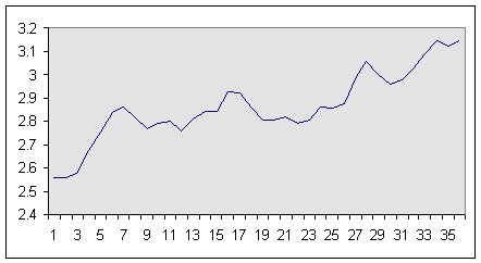
Figure 1: Oil Price, 1994-1996
One can see a fairly clear trend over the part of the series at hand. We don’t claim that you would wish to forecast this series along the average trend observed in the past. However, it would be useful to at least be able to identify what has happened!
Commonly with prices, people take logarithms. This converts constant percentage changes to linear trends (for example, after taking natural logarithms, an annual 1% increase becomes a straight line with slope about 0.01 per year).
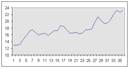
Figure 2: Natural logarithms of Oil Price, 1994-1996
If we took such a series and removed a constant trend, it would be obvious what we had done. In this example we have reduced the values by 10% per annum (roughly 0.8 percent per month). We can get a good idea of the size of the change just by eye (the series diverge by roughly 0.3 in 36 months, which would be about 0.83 percent per month; pretty close for a by-eye measurement).
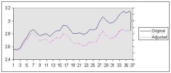
Similarly, if we had adjusted the series with a change in trend that had been 0% for the first 16 months and then 15% per annum after that, we would be able to spot what had been done to the data, again quite easily.
The first difficulty with link ratio methods - cumulating
The link ratio methods commonly used by actuaries for forecasting paid losses begin by adding up (cumulating) the paid losses along accident periods and then calculating link ratios of each partial sum over the previous one. This (as you may see if you try it for yourself with the oil series) makes it far harder to discern any such trend changes as were introduced above, compared to looking at the original series. Below are the first few values of the original and the adjusted series (reduced by 10% per annum), with their cumulated values and the link ratio of each cumulative over the previous one. For example, the link ratio of 1.998 is 25.83/12.93, and that in turn is (12.9+12.93)/12.93.
|
Adjusted
|
|||||||
|
Month
|
Oil Price
|
Cumulated
|
Link Ratio
|
Oil Price
|
Cumulated
|
Link Ratio
|
|
|
1
|
12.93
|
12.93
|
|
12.8277
|
12.83
|
||
|
2
|
12.9
|
25.83
|
1.998
|
|
12.6967
|
25.52
|
1.990
|
|
3
|
13.18
|
39.01
|
1.510
|
|
12.8697
|
38.39
|
1.504
|
|
4
|
14.54
|
53.55
|
1.373
|
|
14.0853
|
52.48
|
1.367
|
|
5
|
15.74
|
69.29
|
1.294
|
|
15.1272
|
67.61
|
1.288
|
|
6
|
17.04
|
86.33
|
1.246
|
|
16.247
|
83.85
|
1.240
|
If we continue the above calculation of link ratios for the whole of the data, we obtain the following plot:
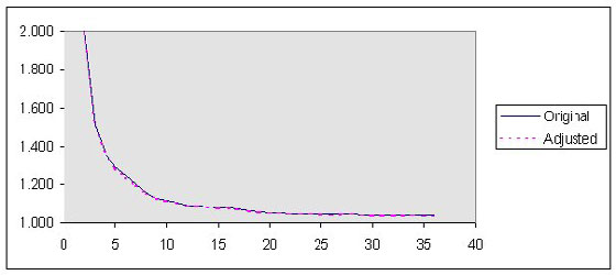
The link ratios for the adjusted series lie below the link ratios for the original series, but not by a constant amount – the adjusted-series link ratios bounce around between 99.52 and 99.63% of the original series link ratios. It is difficult, if not impossible, to see what simple adjustment we made to the data by studying the link ratios. It is even more difficult to discern changing trends.
The second difficulty with link ratio methods - calendar year trends
Paid losses are not single series, but consist of several series (one in respect of each accident year), generally arranged as a table. In the usual triangle formulation, accident years are rows, delay (or development) forms the columns, and calendar time forms diagonals running from lower left to upper right. Any changes that occur in “actual time,” like economic or social effects, occur across that diagonal direction. While they impact on the other two directions, changes in the calendar direction impact each accident year (and development year) at a different point.
Identifying changes in trend
These two kinds of difficulties combine in such a way as to make it effectively impossible to identify changes to trends when using link ratios, as we shall see with a simple example. That inability to identify major calendar period changes (and hence to properly allow for them in the future) is a critical problem with the commonly used link ratio techniques.
An actual paid loss triangle is shown here. These are incremental paid losses for a long tail line of business. We will call the triangle ‘ABC’:
Paid losses, ABC
|
0
|
1
|
2
|
3
|
4
|
5
|
6
|
7
|
8
|
9
|
10
|
||||||||||||
| 1977 | 153,638 | 188,412 | 134,534 | 87,456 | 60,348 | 42,404 | 31,238 | 21,252 | 16,622 | 14,440 | 12,200 | |||||||||||
| 1978 | 178,536 | 226,412 | 158,894 | 104,686 | 71,448 | 47,990 | 35,576 | 24,818 | 22,662 | 18,000 | ||||||||||||
| 1979 | 210,172 | 259,168 | 188,388 | 123,074 | 83,380 | 56,086 | 38,496 | 33,768 | 27,400 | |||||||||||||
| 1980 | 211,448 | 253,482 | 183,370 | 131,040 | 78,994 | 60,232 | 45,568 | 38,000 | ||||||||||||||
| 1981 | 219,810 | 266,304 | 194,650 | 120,098 | 87,582 | 62,750 | 51,000 | |||||||||||||||
| 1982 | 205,654 | 252,746 | 177,506 | 129,522 | 96,786 | 82,400 | ||||||||||||||||
| 1983 | 197,716 | 255,408 | 194,648 | 142,328 | 105,600 | |||||||||||||||||
| 1984 | 239,784 | 329,242 | 264,802 | 190,400 | ||||||||||||||||||
| 1985 | 326,304 | 471,744 | 375,400 | |||||||||||||||||||
| 1986 | 420,778 | 590,400 | ||||||||||||||||||||
| 1987 | 496,200 | |||||||||||||||||||||
Each row represents paid losses for a given accident year (in respect of a particular collection of policies). Each column represents the number of years of delay (sometimes called ‘development’) between the occurrence of the event leading to the claim and when paid losses were made. Each year that passes means that another value is available to add to the end of each row, and if the business is still being written, a new row will be added at the bottom.
This triangle is fairly typical, though it does display an unusually low level of "noise" about the trends in the data. Many paid loss arrays are much more volatile.
The aim with reserving is basically (though there is somewhat more involved in practice) to “fill out” the rest of the table – to predict what the rest of the values will be in each row. It is a little like the 3x3 table used in some IQ tests, where you need to fill in the missing values:
|
10
|
20
|
30
|
|
15
|
30
|
45
|
|
20
|
40
|
?
|
In the little table above, most people would choose “60” as the missing answer. When the patterns are nice and simple like this, it is not difficult to fill out a larger table. Indeed, with simple patterns like these, link ratio methods work – but then almost any reasonable approach will work.
Examples of filling in the missing values
Imagine we had the following triangle of paid losses:
|
1240
|
2728
|
2128
|
1277
|
766
|
|
1240
|
2728
|
2128
|
1277
|
|
|
1240
|
2728
|
2128
|
|
|
|
1240
|
2728
|
|
|
|
|
1240
|
|
|
|
|
If things remain as they have been (no big change in the legal or economic environment, for example), it should cause nobody any difficulty to fill out the rest of the table:
|
1240
|
2728
|
2128
|
1277
|
766
|
|
1240
|
2728
|
2128
|
1277
|
766
|
|
1240
|
2728
|
2128
|
1277
|
766
|
|
1240
|
2728
|
2128
|
1277
|
766
|
|
1240
|
2728
|
2128
|
1277
|
766
|
The usual link ratio methods will work as well.
However, imagine that on top of the simple trends above, there was, impacting the third calendar year and later, an increase in paid losses of 10% per annum:
|
1240
|
2728
|
2341
|
1545
|
1020
|
|
1240
|
3001
|
2575
|
1699
|
|
|
1364
|
3301
|
2832
|
|
|
|
1500
|
3631
|
|
|
|
|
1650
|
|
|
|
The pattern is more complex, but if we follow the “IQ-test” approach, the pattern can soon be discerned. If we work on the log-scale, the pattern is even easier to discern. But the usual link ratio methods have more difficulty. Of course, the numbers here are so regular that an observant actuary will notice that the more recent individual link ratios have changed from the earlier ones:
|
0-1
|
1-2
|
2-3
|
3-4
|
|
3.200
|
1.590
|
1.245
|
1.130
|
|
3.420
|
1.607
|
1.245
|
|
|
3.420
|
1.607
|
|
|
|
3.420
|
|
|
Link ratios cannot detect trend changes in presence of noise
However, in the presence of even quite modest amounts of noise, it is generally not possible to identify that the process has change, even for as dramatic a changed as 10% per annum.
Here are the link ratios for the cumulatives of the triangle ABC given earlier.
ABC: Cumulative Paid Loss Link Ratios
|
0-1
|
1-2
|
2-3
|
3-4
|
4-5
|
5-6
|
6-7
|
7-8
|
8-9
|
9-10
|
||
|
1977
|
2.226 | 1.393 |
1.184
|
1.107
|
1.068 | 1.047 | 1.030 | 1.023 | 1.020 | 1.016 | |
|
1978
|
2.268 | 1.392 |
1.186
|
1.107
|
1.065 | 1.045 | 1.030 | 1.027 | 1.021 | ||
|
1979
|
2.233 | 1.401 |
1.187
|
1.107
|
1.065 | 1.042 | 1.035 | 1.028 | |||
|
1980
|
2.199
|
1.394
|
1.202
|
1.101
|
1.070 | 1.050 | 1.039 | ||||
|
1981
|
2.212 | 1.400 | 1.176 | 1.109 | 1.071 | 1.054 | |||||
|
1982
|
2.229 | 1.387 | 1.204 | 1.126 | 1.096 | ||||||
|
1983
|
2.292 | 1.430 | 1.220 | 1.134 | |||||||
|
1984
|
2.373 | 1.465 | 1.228 | ||||||||
|
1985
|
2.446 | 1.470 | |||||||||
|
1986
|
2.403 |
Here are some link ratios for ABC cumulatives that have been adjusted in some manner along the calendar period direction.
Adjusted ABC: Cumulative Paid Loss Link Ratios
|
0-1
|
1-2
|
2-3
|
3-4
|
4-5
|
5-6
|
6-7
|
7-8
|
8-9
|
9-10
|
||
|
1977
|
2.115 | 1.342 |
1.151
|
1.082
|
1.049 | 1.031 | 1.019 | 1.013 | 1.010 | 1.008 | |
|
1978
|
2.153 | 1.342 |
1.153
|
1.082
|
1.046 | 1.030 | 1.018 | 1.015 | 1.011 | ||
|
1979
|
2.121 | 1.349 |
1.154
|
1.082
|
1.046 | 1.028 | 1.022 | 1.016 | |||
|
1980
|
2.090
|
1.343
|
1.166
|
1.078
|
1.050 | 1.033 | 1.024 | ||||
|
1981
|
2.101 | 1.348 | 1.145 | 1.084 | 1.050 | 1.036 | |||||
|
1982
|
2.117 | 1.337 | 1.167 | 1.097 | 1.069 | ||||||
|
1983
|
2.174 | 1.374 | 1.181 | 1.103 | |||||||
|
1984
|
2.248 | 1.406 | 1.189 | ||||||||
|
1985
|
2.314 | 1.411 | |||||||||
|
1986
|
2.276 |
Can you tell from the numbers what simple adjustment was made? As with the Oil price figures, the link ratios don’t let you see what happened.
Here, the paid loss values were again adjusted by a 10% trend (this time, the values were taken to '1986 dollar' values, assuming economic inflation was actually 10%). The impact on the link ratios in similar to the adjustment that we made to the oil prices. But if we graphed the incremental amounts against time, we could see what was done immediately.
Just as link ratios obscure a simple adjustment, they obscure the changing trends within the data itself. The ABC triangle contains a dramatic trend change in the calendar period direction – in the most recent couple of years the inflation in the paid losses is about 10% higher than it was in most of the data. Because of the low level of volatility in this paid array, a very careful examination of the link ratios can reveal something happened. But it doesn't reveal quite what, or by how much.
The graph below displays the change in trend in the calendar year direction after adjusting for the trends in the other direction, and removing the average change in the calendar direction. It is easy to see the change in trend!
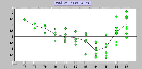
Analysis of the basic trends in the incrementals allows us to rapidly identify this important change. Once we are aware of such an important change, we can begin to ask the right questions; this will allow us to make informed judgments about the future (questions like “What caused this change?”, and the answer to that question would have lead us to ask “Is it a temporary effect which should return to the earlier, lower trend?”). If we do not even recognize this change, we cannot begin to ask the questions, and so we cannot begin to seek the information upon which to make the necessary judgments.
Many actuaries now recognize these and other deficiencies in the use of link ratio approaches to reserving. We have seen that link ratios cannot pick up simple trends and cannot capture trend changes in the paid losses. Another illustration of the problems experienced by link ratios may be found in our paper “When Can Accident Years Be Regarded As Development Years?” (submitted to the CAS Proceedings). It demonstrates that volume- weighted averages do not distinguish at all between accident years and development years. Other weighted link ratios have similar problems, but it is no longer a mathematical identity. And a final, crucial problem - Link Ratios cannot tell you anything about the volatility in paid losses.
To view other papers discussing Claims Reserving and Actuarial Methodologies, click on the following links below.
and
pdf Claims Reserving - Some Thoughts About Principles and Methodologies (182 KB)
Appendix
Refiner Acquisition Cost of Imported Crude Oil. To visit the Energy Information Administration web site click here.
|
Oil Price
|
||||
|
(P)
|
In (P)
|
log 10 (P)
|
||
|
1994
|
Jan
|
12.93
|
2.55955
|
1.111599
|
|
Feb
|
12.9
|
2.557227
|
1.11059
|
|
|
Mar
|
13.18
|
2.578701
|
1.119915
|
|
|
Apr
|
14.54
|
2.676903
|
1.62564
|
|
|
May
|
15.74
|
2.756205
|
1.197005
|
|
|
Jun
|
17.04
|
2.835564
|
1.23147
|
|
|
Jul
|
17.52
|
2.863343
|
1.243534
|
|
|
Aug
|
16.66
|
2.813011
|
1.221675
|
|
|
Sep
|
15.91
|
2.766948
|
1.20167
|
|
|
Oct
|
16.27
|
2.789323
|
1.211388
|
|
|
Nov
|
16.46
|
2.800933
|
1.21643
|
|
|
Dec
|
15.78
|
2.758743
|
1.198107
|
|
|
1995
|
Jan
|
16.56
|
2.80699
|
1.21906
|
|
Feb
|
17.21
|
2.845491
|
1.235781
|
|
|
Mar
|
17.21
|
2.845491
|
1.235781
|
|
|
Apr
|
18.7
|
2.928524
|
1.271842
|
|
|
May
|
18.56
|
2.921009
|
1.26578
|
|
|
Jun
|
17.43
|
2.858193
|
1.241297
|
|
|
Jul
|
16.5
|
2.80336
|
1.217484
|
|
|
Aug
|
16.54
|
2.805782
|
1.218536
|
|
|
Sep
|
16.71
|
2.816007
|
1.22976
|
|
|
Oct
|
16.29
|
2.790551
|
1.211921
|
|
|
Nov
|
16.52
|
2.804572
|
1.21801
|
|
|
Dec
|
17.53
|
2.863914
|
1.243782
|
|
|
1996
|
Jan
|
17.48
|
2.861057
|
1.242541
|
|
Feb
|
17.77
|
2.877512
|
1.249687
|
|
|
Mar
|
19.9
|
2.99072
|
1.298853
|
|
|
Apr
|
21.33
|
3.060115
|
1.328991
|
|
|
May
|
20.12
|
3.001714
|
1.303628
|
|
|
Jun
|
19.32
|
2.961141
|
1.286007
|
|
|
Jul
|
19.6
|
2.97553
|
1.292256
|
|
|
Aug
|
20.53
|
3.021887
|
1.312389
|
|
|
Sep
|
22.04
|
3.092859
|
1.343212
|
|
|
Oct
|
23.22
|
3.145014
|
1.365862
|
|
|
Nov
|
22.66
|
3.120601
|
1.35526
|
|
|
Dec
|
23.22
|
3.145014
|
1.365862
|