In this article, David Munroe and Dr David Odell, illustrate the bootstrap technique with a series of examples beginning from basic principles. The argument commences with a deliberately flawed example to emphasise the importance of verifying that the sample being (directly) bootstrapped (re-sampled) is structureless. That is, the sample is a random sample from the same distribution. It is then shown that if structure remains in the weighted standardised residuals of a fitted model, the bootstrap samples (pseudo-data loss development arrays) can easily be distinguished from the real data, as they do not replicate the features in the real data.
The bootstrap technique is an excellent tool for testing a model, that is, does the model capture the volatility in the data in a parsimoniously.
It is necessary to design a model that carefully splits the trend structure and process variability with the precision of a sushi chef. Cutting incorrectly results in inferior sushi.
The complete article can be downloaded Archive here (5.42 MB) . The "About the Bootstrap" article was published in December 2009 issue of The Actuary UK magazine. Page 30-35.
The following articles are also available:
- Archive The need for diagnostic assessment of bootstrap predictive models (572 KB)
- Some important properties of average link ratio type methods
- The Mack Method and Bootstrap predictions
The need for diagnostic assessment of bootstrap predictive models
The bootstrap is, at heart, a way to obtain an approximate sampling distribution for a statistic (and hence, if required, produce a confidence interval). Where that statistic is a suitable estimator for a population parameter of interest, the bootstrap enables inferences about that parameter. In the case of simple situations the bootstrap is very simple in form, but more complex situations can be dealt with. The bootstrap can be modified in order to produce a predictive distribution (and hence, if required, prediction intervals).
It is predictive distributions that are generally of prime interest to insurers (because they pay the outcome of the process, not its mean). The bootstrap has become quite popular in reserving in recent years, but it's necessary to use the bootstrap with caution.
The bootstrap does not require the user to assume a distribution for the data. Instead, sampling distributions are obtained by resampling the data.
However, the bootstrap certainly does not avoid the need for assumptions, nor for checking those assumptions. The bootstrap is far from a cure-all. It suffers from essentially the same problems as finding predictive distributions and sampling distributions of statistics by any other means. These problems are exacerbated by the time-series nature of the forecasting problem - because reserving requires prediction into never-before-observed calendar periods, model inadequacy in the calendar year direction becomes a critical problem. In particular, the most popular actuarial techniques - those most often used with the bootstrap - don't have any parameters in that direction, and are frequently mis-specified with respect to the behaviour against calendar time.
Further, commonly used versions of the bootstrap can be sensitive to overparameterization - and this is a common problem with standard techniques.
In this paper, we describe these common problems in using the bootstrap and how to spot them.
A basic bootstrap introduction
The bootstrap was devised by Efron (1979), growing out of earlier work on the jackknife. He further developed it in a book (Efron, 1982), and various other papers. These days there are numerous books relating to the bootstrap, such as Efron and Tibshirani (1994). A good introduction to the basic bootstrap may be found in Moore et al. (2003); it can be obtained online.
The original form of the bootstrap is where the data itself is resampled, in order to get an approximation to the sampling distribution of some statistic of interest, in order to make inference about a corresponding population statistic.
For example, in the context of a simple model E(Xi) = μ, i = 1, 2, ... , n, where the X's assumed to be independent, the population statistic of interest is the mean, μ, and the sampling statistic of interest would typically be the sample mean, x_bar .
Consequently, we estimate the population mean by the sample mean (μ_hat = x_bar ) - but how good is that estimate? If we were to collect many samples, how far would the sample means typically be from the population mean?
While that question could be answered if we could directly take many samples from the population, typically we cannot resample the original population again. If we assume a distribution, we could infer the behaviour of the sample mean from the assumed distribution, and then check that the sample could reasonably have come from the assumed distribution.
(Note that rather than needing to assume an entire distribution, if the population variance were assumed known, we could compute the variance of the sample mean, and given a large enough sample, we might consider applying the central limit theorem (CLT) in order to produce an approximate interval for the population parameter, without further assumptions about the distributional form. There are many issues that arise. One such issue is whether or not the sample is large enough - the number of observations per parameter in reserving is often quite small. Indeed, many common techniques have some parameters whose estimates are based on only a single observation! Another issue is that to be able to apply the CLT we assumed a variance - if instead we estimate the variance, then the inference about the mean depends on the distribution again. As the sample sizes become large enough that we may apply Slutzky's theorem, then for example a t-statistic is asymptotically normal, even though in small samples the t-statistic only has a t-distribution if the data were normal. Lastly, and perhaps most importantly when we want a predictive distribution, the CLT usually cannot help.)
In the case of bootstrapping, the sample is itself resampled, and then from that, inferences about the behaviour of samples from the population are made on the basis of those resamples. The empirical distribution of the original sample is taken as the best estimate of the population distribution.
In the simple example above, we repeatedly draw samples of size n (with replacement) from the original sample, and compute the distribution of the statistic (the sample mean) of each resample. Not all of the original sample will be present in the resample - on average a little under 2/3 of the original observations will appear, and the rest will be repetitions of values already in the sample. A few observations may appear more than twice.
The standard error, the bias and even the distribution of an estimator about the population value can be approximated using these resamples, by replacing the population distribution, F by the empirical distribution Fn.
For more complex models, this direct resampling approach may not be suitable. For example, in a regression model, there is a difficulty with resampling the responses directly, since they will typically have different means.
For regression models, one approach is to keep all the predictors with each observation, and sample them together. That is, if X is a matrix of predictors (sometimes called a design matrix) and y is a data-vector, for the multiple regression model Y = XΒ + ε , then the rows of the augmented design matrix [X|y] are resampled. (This is particularly useful when the X's are thought of as random.)
A similar approach can be used when computing multivariate statistics, such as correlations.
Another approach is to resample the residuals from the model. The residuals are estimates of the error term, and in many models the errors (or in some cases, scaled errors) at least share a common mean and variance. The bootstrap in this case assumes more than that - they should have a common distribution (in some applications this assumption is violated).
In this case (with the assumption of equal variance), after fitting the model and estimating the parameters, the residuals from the model are computed: ei = yi - y_hati , and then the residuals are resampled as if they were the data.
Then a new sample is generated from the resampled residuals by adding them to the fitted values, and the model is fitted to the new bootstrap sample. The procedure is repeated many times.
Forms of this residual resampling bootstrap have been used almost exclusively in reserving.
If the model is correct, appropriately implemented residual resampling works. If it is incorrect, the resampling scheme will be affected by it, some more than others, though in general the size of the difference in predicted variance is small. More sophisticated versions of this kind of resampling scheme, such as the second bootstrap procedure in Pinheiro et al. (2003) can reduce the impact of model misspecification when the prediction is, as is common for regression models, within the range of the data. However, the underlying problem of amplification of unfitted calendar year effects remains, as we shall see.
For the examples in this paper we use a slightly augmented version of Sampler 2 given in Pinheiro et al - the prediction errors are added to the predictions to yield bootstrap-simulated predictive values, so that we can directly find the proportion of the bootstrap predictive distribution below the actual values in one-step-ahead predictions.
In the case of reserving, the special structure of the problem means that while often we predict inside the range of observed accident years, and usually also within the range of observed development years, we are always projecting outside the range of observed calendar years - precisely the direction in which the models corresponding to most standard techniques are inadequate.
As a number of authors have noted, the chain ladder models the data using a two-way cross-classification scheme (that is, like a two-way main-effects ANOVA model in a log-link). As discussed in Barnett et al. (2005), this is an unsuitable approach in the accident and development direction, but the issues in the calendar direction are even more problematic. Even the more sophisticated approaches to residual resampling can fail on the reserving problem if the model is unsuitable.
Diagnostic displays for a bootstrapped chain ladder
Many common regression diagnostics for model adequacy relate to analysis of residuals, particularly residual plots. In many cases these work very well for examining many aspects of model adequacy. When it comes to assessing predictive ability, the focus should, where possible, shift to examining the ability to predict data not used in the estimation. In a regression context, a subset of the data is held aside and predicted from the remainder. Generally the subset is selected at random from the original data. However, in our case, we cannot completely ignore the time-series structure and the fact that we're predicting outside the range of the data. Our prediction is always of future calendar time. Consequently the subsets that can be held aside and assessed for predictive ability are those at the most recent time periods.
This is common in analysis of time series. For example, models are sometimes selected so as to minimize one-step-ahead prediction errors. See, for example, Chatfield (2000).
Out of sample predictive testing
The critical question for a model being used for prediction is whether the estimated model can predict outside the sample used in the estimation. Since the triangle is a time series, where a new diagonal is observed each calendar period, prediction (unlike predictions for a model without a time dimension) is of calendar periods after the observed data. To do out-of-sample tests of predictions, it is therefore important to retain a subset of the most recent calendar periods of observations for post-sample predictive testing. We refer to this post-sample-predictive testing as model validation (note that some other authors use the term to mean various other things, often related to checking the usefulness or appropriateness of a model).
Imagine we have data up to time t. We use only data up to time t-k to estimate the model and predict the next k periods (in our case, calendar periods), so that we can compare the ability of the model to predict actual observations not used in the estimation. We can, for example, compute the prediction errors (or validation residuals), the difference between observed and predicted in the validation period. If these prediction errors are divided by the predictive standard error, the resulting standardized validation residuals can be plotted against time (calendar period most importantly, and also accident and development period), and against predicted values, (as well as against any other likely predictor), in similar fashion to ordinary residual plots. Indeed, the within-sample residuals and "post-sample" predictive errors (validation residuals) can be combined into a single display.
One step ahead prediction errors are related to validation residuals, but at each calendar time step only the next calendar period is predicted; then the next period of data is brought in and another period is predicted.
In the case of ratio models such as the chain-ladder, prediction is only possible within the range of accident and development years used in estimation, so out of sample prediction cannot be done for all observations left out of the estimation. The use of one step ahead prediction errors maximizes the number of out-of-sample cases that have predictions. Further, when reserving, the liability for the next calendar period is generally a large portion of the total liability, and the liability estimated will typically be updated once it is observed; this makes one-step-ahead prediction errors a particularly useful criterion for model evaluation when dealing with ratio models like the chain ladder.
For a discussion of the use of out of sample prediction errors and in particular one-step-ahead prediction errors in time series, see Chatfield (2000), chapter 6.
For many models, the patterns in residual plots when compared with the patterns in validation residuals or one step ahead prediction errors appear quite similar. In this circumstance, ordinary residual plots will generally be sufficient for identifying model inadequacy.
Critically, in the case of the Poisson and quasi-Poisson GLM that reproduce the chain ladder, the prediction errors and the residuals do show different patterns.
Example 1:
See Appendix A. This data was used in Mack (1994). The data are incurred losses for automatic facultative business in general liability, taken from the Reinsurance Association of America's Historical Loss Development Study.
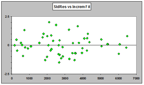
If we fit a quasi- (or overdispersed) Poisson GLM and plot standardized residuals against fitted values, the plot appears to show little pattern:
However, if we plot one step ahead prediction errors (scaled by dividing the prediction errors by μ_hat1/2 ) against predicted values, we do see a distinct pattern of mostly positive prediction errors for small predictions with a downward trend toward more negative prediction errors for large predictions:
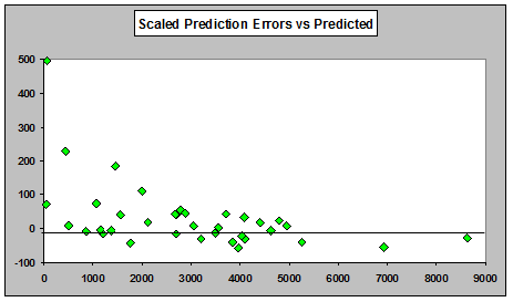
Prediction errors above have not been standardized to have unit variance. The underlying quasi-Poisson scale parameter would have a different estimate for each calendar year prediction; it was felt that the additional noise from separate scaling would not improve the ability of this diagnostic to show model deficiencies. On the other hand, using a common estimate across all the calendar periods would simply alter the scale on the right hand side without changing the plot at all, and has the disadvantage that for many predictions you'd have to scale them using "future" information. On the whole it seems prudent to avoid the scaling issue for this display, but as a diagnostic tool, it's not a major issue.
This problem of quite different patterns for prediction errors and residuals does not tend to occur with the Mack formulation of the chain ladder, where ordinary residuals are sufficient to identify this problem:
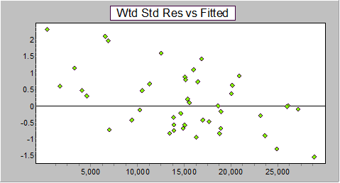
As noted in Barnett and Zehnwirth (2000), this is caused by a simple failure of the ratio assumption - it is not true that E(Y|X) = ΒX, as would be true of any model where the next cumulative is assumed to be (on average) a multiple of the previous one. (For this data, the relationship between Y and X does not go through the origin.)
The above plot is against cumulatives because in the Mack formulation, that's what is being predicted. For comparison, here are the OD Poisson GLM residuals vs cumulative fitted rather than incremental fitted:
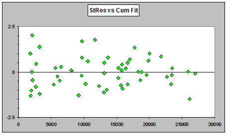
Why is the problem obvious in the residuals for the Mack version of the chain ladder model, but not in the plots of GLM residuals vs fitted (either incremental or cumulative)? Even though the two models share the same prediction function, the fitted values of the two models are different.
On the cumulative scale, if X is the most recent cumulative (on the last diagonal) and Y is the next one, both models have the prediction-function E(Y|X) = ΒX.
Within the data, the Mack model uses the same form for the fit - E(Y|X) = ΒX, but the GLM does not - you can write it as E(Y) = ΒE(X), which seems similar enough that it might be imagined it would not make much difference, but the right hand side involves "future" values not available to predictions. This allows the fit to "shift" itself to compensate, so you can't see the problem in the fits. However, the out-of-sample prediction function is the same as for the Mack formulation, and so the predictions from the GLM suffers from exactly the same problem - once you forecast future values, you're assuming E(Y|X) = ΒX for the future - and it does not work.
Adequate model assessment of ODP GLMs therefore requires the use of some form of out-of-sample prediction, and because of the structure of the chain ladder, this assessment seems to be best done with one-step-ahead prediction errors. For many other models, such as the Mack model, this would be useful but not as critical, since we can identify the problem even in the residuals.
Assessing bootstrap predictive distributions
When calculating predictive distributions with the bootstrap, we can in similar fashion make plots of standardized prediction errors against predicted values and against calendar years. Of course, since the prediction errors are the same, the only change would be a difference in the amount by which each prediction error is scaled (since we have bootstrap standard errors in place of asymptotic standard errors from an assumed model); the broad pattern will not change, however, so the plot based on asymptotic results are useful prior to performing the bootstrap.
Since we can produce the entire predictive distribution via the bootstrap, we can evaluate the percentiles of the omitted observations from their bootstrapped predictive distributions - if the model is suitable, the data should be reasonably close to "random" percentiles from the predictive distribution. This further information will be of particular interest for the most recent calendar periods (since the ability of the model to predict recent periods gives our best available indication if there is any hope for it in the immediate future - if your model cannot predict last year you cannot have a great deal of confidence in its ability to predict next year).
We could look at a visual diagnostic, such as the set of predictive distributions with the position of each value marked on it, though it may be desirable to look at all of them together on a single plot, if the scale can be rendered so that enough detail can be gleaned from each individual component. It may be necessary to "summarize" the distribution somewhat in order to see where the values lie (for example, indicating 10th, 25th, 50th, 75th and 90th percentiles, rather than showing the entire bootstrap density). In order to more readily compare values it may help to standardize by subtracting the mean and dividing by the standard deviation, though in many cases, if the means don't vary over too many standard deviations, simply looking at the original predicted values on (whether on the original scale or on a log scale) may be sufficient - sometimes a little judgement is required as to which plot will be most informative.
In some circumstances it might also be useful to obtain a single summary of the indicated lack of 'predictive fit'. If the data are "random" percentiles from their predictive distributions, the proportion of the predictive distribution below which each observation falls should be uniform. Of primary interest would be (i) substantial bias in the predictive distribution (both up and down bias are problematic for the insurer), and (ii) substantial error in the variability of the predictive distribution. The first will tend to yield percentiles that are too high or too low, which the second will either yield percentiles that are both too high and too low (if the predictive variance is underestimated), or percentiles that are clustered toward the centre (if it is overestimated). If pi is the proportion of the predictive distribution below the observed value, then qi = 2| pi - 1/2 | should also be uniform, but if there are too many extreme percentiles (either from upward or downward bias, or from underestimating of the predictive variances), the qi values will tend to be too large, while if there are too few extreme percentiles the qi values will tend to be too small. There are various ways of combining the qi into a single diagnostic measure. Once such would be to note that if the q's are uniform, then 2.exp(-{1-qi}) has a chi-square distribution with 2d.f. (with large values again indicating an excess of extreme percentiles). Several of these (k, say) may be added if a single statistic is desired and compared with a Χ22k distribution. Unusually large values would be of particular interest, though unusually small values would also be important. If required this could be used as a formal hypothesis test, but it is generally of greater value as a diagnostic summary of the overall tendency to extreme percentiles.
Example 2
ABC data. This is Worker's Compensation data for a large company. This data was analyzed in some detail in Barnett and Zehnwirth (2000). See appendix B.
In this example we actually use the bootstrap predictions discussed in the basic bootstrap introduction above, based on the second algorithm from Pinheiro et al (2003). Below are the predictive distributions for the first two values (after DY0) for the last diagonal, for a ODP GLM fitted to the data prior to the final calendar year, which was omitted. The brown arrows mark the actual observation that the predictive distribution is attempting to predict.
ABC Predictive distribution for last diagonal - histograms
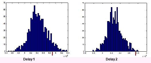
The arrow marks the actual observation for that delay; for the two distributions shown, the observed value sits fairly high. For a single observation, this might happens by chance, even with an appropriate model, of course.
The runoff decreases sharply for this triangle, so most of this information in the histograms would be lost if we looked at them on a single plot. Consequently, for a more detailed examination, the bootstrap results are reduced to a five-number summary of the percentiles:
ABC Predictive distribution for last diagonal - box and whisker plots
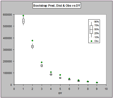
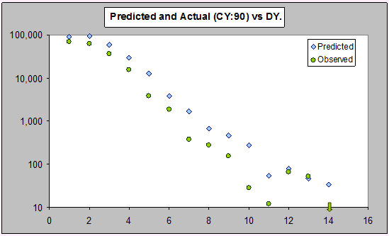
As can be seen, the actual payments for the first seven development periods are all very high, but it's a little hard to see the details in the last few periods. Let's look at them on the log-scale:
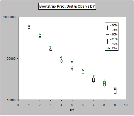
Now we can see that in all cases the observations sit above the median of the predictive distribution, and all but the last two are above the upper quartile.
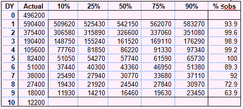
Below is a summary table of the bootstrap distribution for the final calendar year:
ABC: Bootstrap Predictive distributions for last calendar year
So what's going on? Why is this predicting so badly?
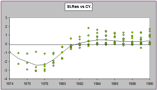
Well, we can see via one-step ahead prediction errors that there's a problem with the assumption of no calendar period trend; alternatively, as we noted earlier, we can look at residuals from a Mack-style model, and get a similar impression:
We can see a strong trend-change. Consequently, predictions of the last calendar year will be too low. One major difficulty with the common use of the chain ladder in the absence of careful consideration of the remaining calendar period trend is that there is no opportunity to apply proper judgement of the future trends in this direction, because the practitioner lacks information about the past behaviour for a context in which to even seek information that would inform scenarios relating to the future behaviour.
Example 3 - LR high
The data for this example is available in Appendix C. As we have seen, we can look at diagnostics and assess before we attempt to produce bootstrap prediction intervals whether we should proceed.
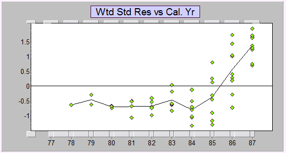
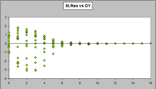
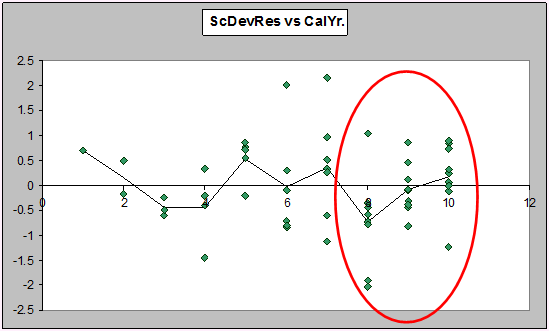
Here are the standardized residuals vs calendar years from a Mack-style Chain ladder fit. As you can see, there's a lot of structure.
There's similar structure in the overdispersed Poisson GLM formulation of the chain ladder - residuals show there are strong trend changes in the calendar year direction:
However, as we described before, this residual plot gives the incorrect impression that the GLM is underpredicting. This impression is incorrect, as we see by looking at the validation (one step ahead predictions) for the last year:
It's a little hard to see detail over on the right, so let's look at the same plot on the log scale:
The Mack-model residual plot gave a good indication of the predictive performance of the chain ladder (bootstrapped or not) for both the Mack model and the quasi- (overdispersed) Poisson GLM. It's always a good idea to validate the last calendar year (look at one-step-ahead prediction errors), but a quick approximation of the performance is usually given by examining residuals from a Mack-chain ladder model.
A further problem with the GLM is revealed by the plot of residuals vs development year:
The assumed variance function does not reflect the data.
Example 4
The next example has been widely used in the literature relating to the chain ladder. Indeed, Pinherio et al. (2003) referred to it as a "benchmark for claims reserving models". The data come from Taylor and Ashe (1983). See Appendix D.
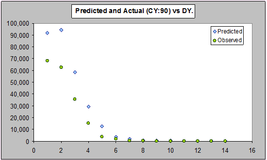
Here are the bootstrap predictive means and s.d.s for the last diagonal (i.e. with that data not used in the estimation) for a quasi-Poisson GLM, and the actual payments for comparison:
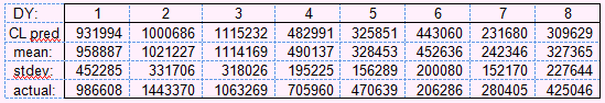
Firstly, there is an apparent bias in the bootstrap means. The chain ladder predictions sit below the bootstrap means, indicating a bias. Since, the ML for a Poisson is unbiased, if the model is correct, these predictions should be unbiased. This doesn't necessarily indicate a bad predictive model, but is there anything going on?
In fact there is, and we can see problem can be seen in residual plots.
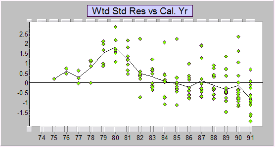
Here is a plot of the residuals versus calendar year from a Mack type fit (this is done first because it's the easiest to obtain - it takes only a couple of clicks in ICRFS-ELRF).
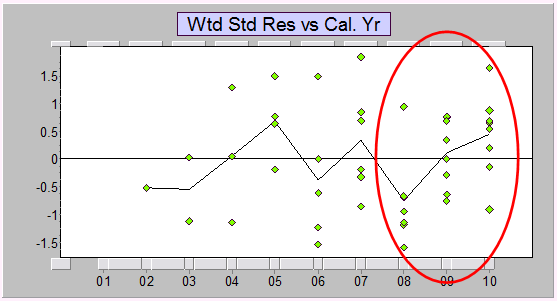
Strong calendar period effects in the last few years. The existence of a calendar period effect was already noted by Taylor and Ashe in 1983 (who included the late calendar year effect in some of their models), but it has been ignored by almost every author to consider this data since. If the trend were to continue for next year, the forecasts may be quite wrong. If we didn't examine the residuals, we may not even be aware this problem is present.
Exactly the same effect appears when fitting a quasi-Poisson two-way cross classification with log-link:
There's little advantage in not examining Mack residuals before fitting a quasi-Poisson GLM - the residuals are easier to produce, and the information in the plot of residuals vs fitted has more information about the predictive ability of the model.
Some other considerations
All chain-ladder reproducing models (including both the quasi-Poisson GLM and the Mack model) must assume that the variance of the losses is proportional to the mean (or they will necessarily fail to reproduce the chain ladder). This assumption is found to be rarely tenable in practice - and for an obvious reason. While it can make sense with claim counts - for example, if the counts are higher on average they also tend to be more spread but often with lower coefficient of variation. If they happen to be Poisson-distributed (a strong assumption), the variance will be specifically proportional to the mean. However, heterogeneity or dependence in claim probabilities can make it untenable even for claim numbers. But with claim payments, the amount paid on each claim is itself a random variable, not a constant, and anything that makes the claim payments variable will make the variation increase faster than the mean. Simple variation in claim size (such as a constant percentage change, whether due to inflation effects or change in mix of business or any number of other effects) will make the variance increase as the square of the mean, while claim size effects that vary from policy to policy can make it increase still faster. Dependence in claim size effects across policies can make it increase faster again. Consequently the chain ladder assumption of variance proportional to mean must be viewed with a great deal of caution, and carefully checked.
The chain ladder model is overparameterized. It assumes, for example, that there is no information in nearby development periods about the level of payments in a given development, yet the development generally follows a fairly smooth trend - indicating that there is information there, and that the trend could be described with few parameters. This overparameterization leads to unstable forecasts.
Finally, in respect of the bootstrap, the sample statistic may in some circumstances be very inefficient as an estimator of the corresponding population quantities. It would be prudent to check that it makes sense to use the estimator you have in mind for distributions that would plausibly describe the data.
Conclusions
The use of the bootstrap does not remove the need to check assumptions relating to the appropriateness of the model. Indeed, it is clear that there's a critical need to check the assumptions.
The bootstrap cannot get around the facts that chain-ladder type models have no simple descriptors of features in the data. Note further for triangles ABC and LR-High there is so much remaining structure in the residuals -the bootstrap cannot get around this.
If you do fit a quasi-Poisson GLM, it's important to check the one-step-ahead prediction errors in order to see how it performs as a predictive model - the residuals against fitted values don't show you the problems.
In any case, it should be looked at before bootstrapping a model, and once a bootstrap has been done, you should also validate at least the last year - examine whether the actual values from the last calendar year could plausibly have come from the predictive distribution standing a year earlier.
If it is the predictive behaviour that is of interest, prediction errors are appropriate tools to use in standard diagnostics, and they can be analyzed in the same way as residuals are for models where prediction is within the range of the data.
Checking the model when bootstrapping is achieved in much the same way as it is for any other model - via diagnostics - but they must be diagnostics selected with a clear understanding of the problem, the model and the way in which the bootstrap works.
References
Ashe F. (1986), An essay at measuring the variance
Barnett, G., Zehnwirth, B. and Dubossarsky, E. (2005) When can accident years be regarded as development years?
www.casact.org/pubs/proceed/proceed05/05249.pdf
Chatfield, C. (2000), Time Series Forecasting, Chapman and Hall/CRC Press
Efron, B. (1979) Bootstrap methods: another look at the jackknife, Ann. Statist., 7, 1-26.
Efron, B. (1982) The Jacknife, the Bootstrap and Other Resampling Plans. vol 38, SIAM, Philadelphia.
Efron, B. and Tibshirani, R. (1994) An Introduction to the Bootstrap, Chapman and Hall, New York.
England and Verrall (1999) Analytic and bootstrap estimates of prediction errors in claims reserving, Insurance: Mathematics and Economics, 25, 281-293.
Mack, Th. (1994), "Which stochastic model is underlying the chain ladder method?", Insurance Mathematics and Economics, Vol 15 No. 2/3, pp. 133-138.
Moore, D. S., G.P. McCabe, W.M. Duckworth, and S.L. Sclove (2003), "Bootstrap Methods and Permutation Tests," companion chapter 18 to The Practice of Business Statistics, W. H. Freeman (also 2003).
Pinheiro, P.J.R., Andrade e Silva , J. M. and Centeno, M. L. (2003) Bootstrap Methodology in Claim Reserving, Journal of Risk and Insurance, 70 (4), pp. 701-714
Reinsurance Association of America (1991), Historical Loss Development Study, 1991 Edition, Washington, D.C.: R.A.A.
Taylor, G.C. and Ashe, F.R. (1983) Second Moments of Estimates of Outstanding Claims, Journal of Econometrics, 23, pp 37-61.